Large Language Models (LLMs) are remarkable at reasoning over the text you give them, but they have two hard limitations. One, their knowledge is frozen at training time, and second their context window can only hold so much. Vector stores are the piece of infrastructure that works around both problems, and they sit at the heart of retrieval-augmented generation (RAG), semantic search, and long-term memory for AI agents. This post covers what vector stores are, why they exist, and how they fit into an LLM application.
From Text to Vectors: Embeddings
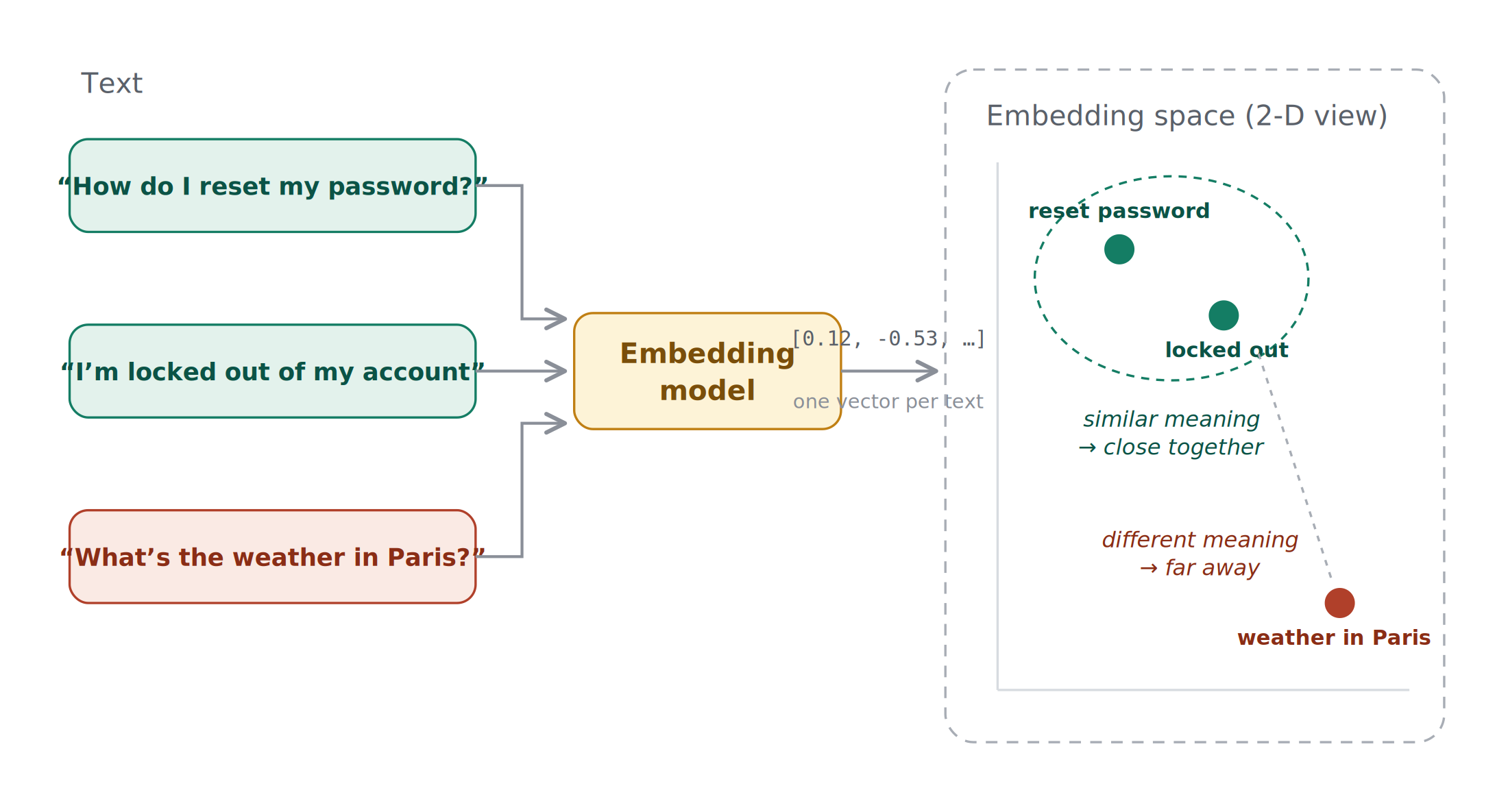
Before we can talk about vector stores, we need embeddings. An embedding model takes a piece of text (a word, sentence, paragraph, or document chunk) and maps it to a dense vector of floating-point numbers, typically with 384 to 3,072 dimensions. The crucial property is that semantic similarity becomes geometric proximity: texts that mean similar things end up close together in this high-dimensional space, even if they share no words.
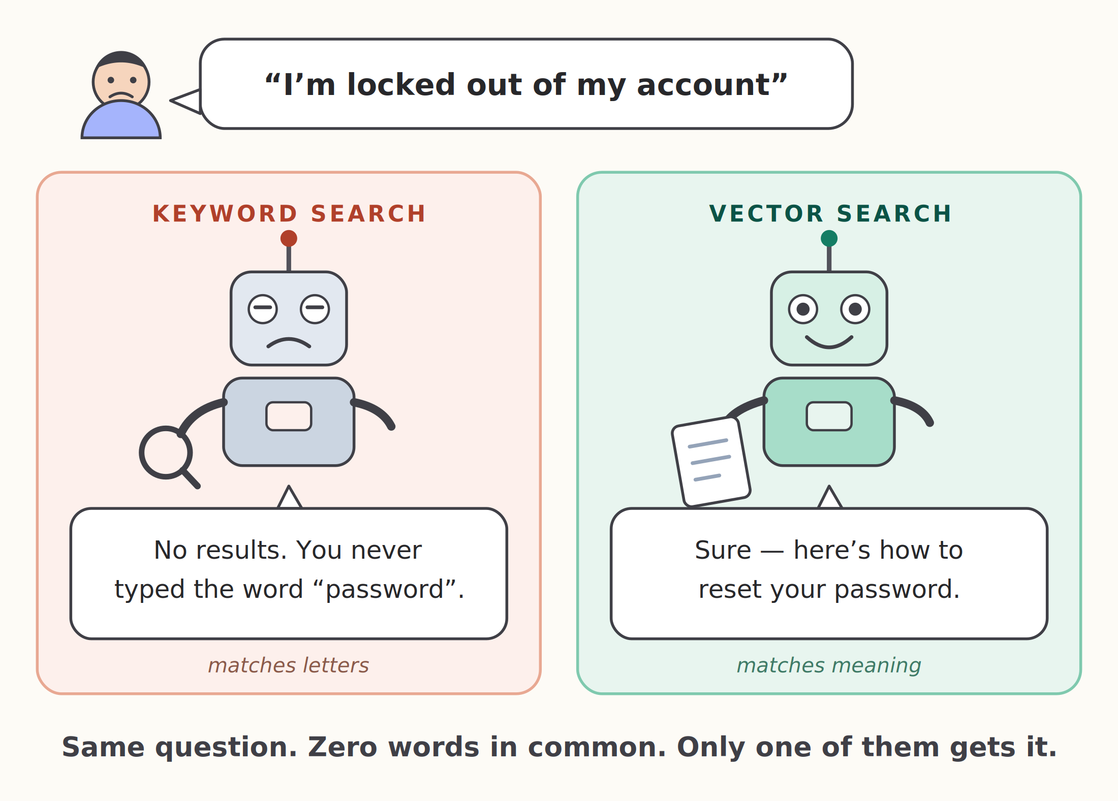
For example, “How do I reset my password?” and “I’m locked out of my account” will produce nearby vectors, while “What’s the weather in Paris?” lands somewhere far away. This is what makes embeddings so much more powerful than keyword search for many use cases.
What Is a Vector Store?
A vector store (or vector database) is a system purpose-built to:
- Store large collections of embedding vectors, usually alongside the original text and metadata (source, timestamp, author, tags).
- Index those vectors so that similarity search is fast.
- Query by taking a new vector and returning the k nearest neighbors — the stored items most similar to the query.
Similarity is measured with metrics like cosine similarity, dot product, or Euclidean distance . Cosine similarity is the most common choice for text embeddings because it focuses on the direction of vectors rather than their magnitude.
Why Not Just Brute-Force It?
Comparing a query vector against every stored vector (exact nearest-neighbor search) is perfectly fine for a few thousand items. But at millions or billions of vectors, a linear scan becomes too slow for interactive applications.
Vector stores solve this with approximate nearest neighbor (ANN) indexes, which trade a small amount of recall for enormous speedups. The most common approaches are:
- HNSW (Hierarchical Navigable Small World) — a graph-based index where search hops between connected nodes, narrowing in on the neighborhood of the query. Fast and accurate; the default in many systems.
- IVF (Inverted File Index) — clusters the vector space and only searches the clusters closest to the query.
- Product Quantization (PQ) — compresses vectors to reduce memory footprint, often combined with IVF.
As a user of a vector store you rarely implement these yourself, but understanding the trade-offs (speed vs. recall vs. memory) helps you tune parameters like ef_search or the number of probed clusters.
The RAG Pipeline: Where Vector Stores Fit
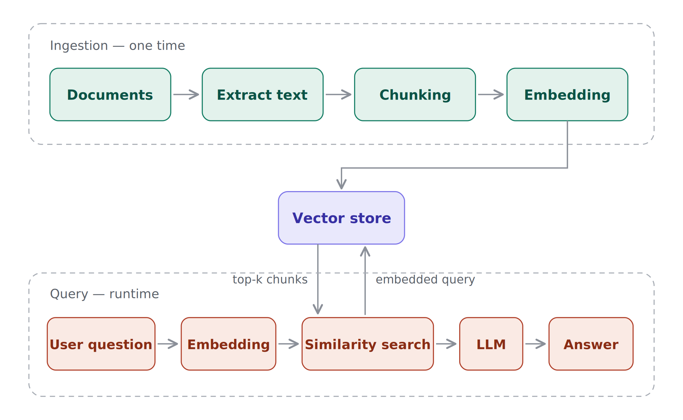
The canonical use case is retrieval-augmented generation. The flow looks like this:
Ingestion (offline):
- Collect your documents (wikis, PDFs, Word Docs, slides, code).
- Split them into chunks — commonly a few hundred tokens each, often with some overlap so ideas aren’t cut mid-thought.
- Embed each chunk with an embedding model.
- Write the vectors, original text, and metadata into the vector store.
Query time (online):
- The user asks a question.
- Embed the question with the same embedding model.
- Query the vector store for the top-k most similar chunks.
- Assemble those chunks into the LLM’s prompt as context.
- The LLM answers grounded in the retrieved material.
Note that the embedding model appears in both diagrams — it must be the same model on both sides, since vectors from different models aren’t comparable. The result is that the model can now answer questions about private, recent, or domain-specific data it was never trained on, and it can cite its sources.
Metadata Filtering and Hybrid Search
Real applications rarely rely on pure vector similarity alone.
- Metadata filtering lets you constrain a search: “only documents from the engineering wiki, updated after January, visible to this user.” Most vector stores support filtered ANN search natively.
- Hybrid search combines dense vector search with traditional keyword search (like BM25). Keyword search excels at exact matches — product codes, error strings, names — whereas embeddings can be fuzzy. Scores from both are merged, often with reciprocal rank fusion.
- Reranking is a common final step: a cross-encoder model re-scores the top candidates for better precision before they reach the LLM.
The Landscape
Options range from lightweight libraries to managed services:
- Libraries: FAISS, hnswlib, and usearch give you raw ANN indexes you manage yourself.
- Dedicated vector databases: Pinecone, Weaviate, Qdrant, Milvus, and Chroma offer persistence, filtering, replication, and APIs out of the box.
- Extensions to existing databases: pgvector for Postgres, along with vector support in Elasticsearch, OpenSearch, Redis, and MongoDB. These are attractive when you already run the underlying database and want to avoid another system.
For prototypes, an in-process option like Chroma or FAISS is often enough. For production, the decision usually comes down to scale, filtering needs, operational preferences, and whether you want vectors living next to your existing data.
Hands-On with a Local Vector Store
Let’s make this concrete with Chroma, an open-source vector store that runs entirely on your machine (no server, no API keys, no Docker). Paired with a small local embedding model from sentence-transformers, you get a complete semantic search pipeline in one script.
|
1 2 |
pip install chromadb sentence-transformers |
We’ll use all-MiniLM-L6-v2 as the embedding model: it produces 384-dimensional embeddings (the low end of the range mentioned earlier), is built on Microsoft’s MiniLM architecture, was fine-tuned for sentence embeddings by the sentence-transformers project, and is released under the Apache 2.0 license — free for commercial use and fully self-hostable.
|
1 2 3 4 5 6 7 8 9 10 11 12 13 14 15 16 17 18 19 20 21 22 23 24 25 26 27 28 29 30 31 32 33 34 35 36 37 38 39 40 |
import chromadb from sentence_transformers import SentenceTransformer # 1. Load a small, fast local embedding model (~80 MB, downloads once) model = SentenceTransformer("all-MiniLM-L6-v2") # 2. Create a persistent vector store on disk client = chromadb.PersistentClient(path="./chroma_db") collection = client.get_or_create_collection( name="knowledge_base", metadata={"hnsw:space": "cosine"}, # use cosine similarity ) # 3. Ingest: embed some document chunks and store them with metadata docs = [ "Employees accrue 20 days of paid vacation per year.", "Password resets are handled through the self-service portal at id.example.com.", "The deploy pipeline runs tests, builds a container, and pushes to staging.", "Expense reports must be submitted within 30 days of purchase.", "Production incidents are triaged in the #incident-response channel.", ] collection.add( ids=[f"doc-{i}" for i in range(len(docs))], documents=docs, embeddings=model.encode(docs).tolist(), metadatas=[ {"source": "hr"}, {"source": "it"}, {"source": "eng"}, {"source": "hr"}, {"source": "eng"}, ], ) # 4. Query: embed the question and find the most similar chunks question = "I'm locked out of my account, what do I do?" results = collection.query( query_embeddings=model.encode([question]).tolist(), n_results=2, ) for doc, dist in zip(results["documents"][0], results["distances"][0]): print(f"{dist:.3f} {doc}") |
Sample output (exact distances will vary slightly by library and model version):
|
1 2 |
0.518 Password resets are handled through the self-service portal at id.example.com. 0.964 Employees accrue 20 days of paid vacation per year |
Notice what happened: the query says “locked out of my account” and the top result talks about “password resets” — zero words in common, yet the store surfaced the right document because their embeddings are close. The distance column (lower = more similar with cosine distance) shows the password doc is a much stronger match than the runner-up.
Two things worth trying from here:
Metadata filtering. Constrain the search to a subset of documents:
|
1 2 3 4 5 |
results = collection.query( query_embeddings=model.encode([question]).tolist(), n_results=2, where={"source": "it"}, # only search IT docs ) |
Closing the RAG loop. To turn this into retrieval-augmented generation, take the retrieved chunks and hand them to an LLM:
|
1 2 3 |
context = "\n".join(results["documents"][0]) prompt = f"Answer using only this context:\n{context}\n\nQuestion: {question}" # send `prompt` to your LLM of choice |
Because we used PersistentClient, everything is saved to ./chroma_db — restart the script and your data is still there. That’s the entire mechanical core of a RAG system; production versions add better chunking, hybrid search, and reranking on top of this same skeleton.
Practical Tips
- Chunking matters more than you’d expect. Too small and chunks lack context; too large and retrieval gets noisy and eats your context window. Start around 300–800 tokens and iterate.
- Use the same embedding model for indexing and querying. Vectors from different models live in incompatible spaces.
- Store the source text and metadata with the vector. You’ll need it for prompt assembly and citations.
- Measure retrieval quality separately from generation quality. If the right chunks aren’t retrieved, no amount of prompt engineering will fix the answer.
- Plan for re-indexing. Switching embedding models means re-embedding your entire corpus, so keep raw documents accessible.
Wrapping Up
Vector stores turn the fuzzy notion of “meaning” into something you can index and query at scale. Paired with embeddings and an LLM, they form the retrieval backbone that lets AI systems work with knowledge that is private, fresh, and far larger than any context window. Understand embeddings, ANN indexing, and the RAG pipeline, and you understand the essential mechanics of most LLM applications shipping today.